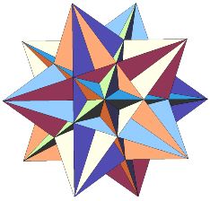
Figure 1
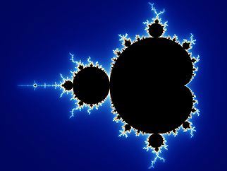
Figure 2
Geometric Structures: Session I
Pleasing Shapes, Careful Looking, Same-Different, and the Power of Words
Prepared by:
Joseph Malkevitch
Department of Mathematics
York College (CUNY)
Jamaica, New York 11451
email:
malkevitch@york.cuny.edu
web page:
http://york.cuny.edu/~malk
Pleasing shapes
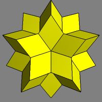
Our daily lives are enriched by pleasing shapes:
Some shapes are pleasing because they are so symmetrical and other shapes are pleasing because they are so complicated.
Shapes are the concern of the area of mathematics called geometry. However, here we will adopt a broader view of geometry, which can be thought of as the science of studying visual patterns. Shapes are only one part of the story.
Careful Looking
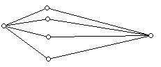
Take a careful look at the shape below, which you should think of as being a drawing in the plane (flat surface) of an object in 3 dimensions.
Do now 1:
a. Write down on a piece of paper a list of as many properties or facts about the object (Figure 3) as you can. (Minimum 5)
b. Exchange your list with the person sitting next to you. Use the list of your neighbor to help you add 5 new additional properties to your original list.
When one looks at shapes and wants to describe them to other people, one uses words. Some of the words that might be used in describing the object in Figure 1 are:
Corners
Sides
Edges
Polyhedron
Flat
Polygon
Faces
Congruent
Regions
Pentagon
Vertices
Immediately you may realize that different people may use different words for the same thing. Also different people may use the same word but have different meanings in mind - and I will restrict myself to only using words in English. Furthermore, sometimes words that we use in common everyday language may be used in a different way from the way that these terms are used in mathematics.
Exercise 1
Practice careful looking at these objects:
a.

Here I will try to show that historically the evolution of the meaning of words has helped drive the creation of new mathematics. For example, all of the diagrams in Figure 6 would today be called polygons, but at times in the past this would not have been true!
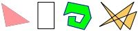
Figure 6 illustrates convex 3-gons and 4-gons and a non-convex polygon with 12 sides, as well as a self-intersecting polygon with 6 sides. Sometimes it will be convenient to think of polygons as points (vertices) joined by rods, and sometimes as filled in regions with a certain number of sides. I will refer to these as rod and membrane models for the polygon concept. When one thinks of a polygon as a system of "rods," it is still customary to refer to a polygon such as the 4-gon in Figure 6 as convex. The usual definition of a convex set is that a set X is convex if for any two points p and q in X the line segment joining p and q is also in X. Strictly speaking, if one is thinking of the 4-gon in Figure 6 as a collection of rods, one should say that this polygon together with its interior points is convex.
One of the most fundamental properties of the Euclidean plane is that if one draws a polygon which does not intersect itself such as the one in Figure 7, then the polygon divides the plane into three sets: those points on the polygon, those points in the interior of the polygon, and those points in the exterior of the polygon.
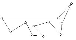
This fact (generalized to curves rather than polygons) is known as the Jordan Curve Theorem and is named for the French topologist Camille Jordan.
Many of the shapes we will be interested in studying can be understood with the help of a geometric tool called a graph. A graph is a diagram (Figure 8) consisting of dots called vertices (the singular is vertex) which are joined by line segments, which may be straight or curved, called edges.
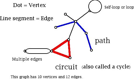
The valence of a vertex where there is no self-loop is the number of distinct edges at the vertex. A self-loop contributes two (2) to the valence of the vertex it is located at. In the graph above, the vertex where the self-loop appears has valence 3. The other vertices which are not 1-valent (there are three 1-valent vertices in this graph) have valences 5, 4, 3, 2, 2 and 2. Thus, a complete list of the valences for this graph is: 5, 4, 3, 3, 2, 2, 2, 1, 1, 1. The sum of the valences in a graph is twice the number of edges in the graph. Another name for the valence of a vertex is degree of a vertex. Computer scientists often refer to vertices with valence 1 as the leaves of a graph. The path shown has length 3 and the circuit also has length 3. Note that this graph (Figure 8) has been drawn in the plane so that edges in the graph meet only at vertices. Drawings of this kind are known as plane drawings.
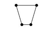
Sometimes, with advantage, the same object can be looked at from different points of view. For example, the diagram in Figure 9 can be thought of as a polygon with 4 sides and also as a graph with 4 vertices and 4 edges.
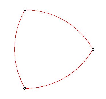
The diagram in Figure 10 shows a shape which I will not consider a polygon because its sides are not portions of straight lines. For this particular shape, the graph associated with the shape would still be a 3-gon, just the way a triangle's graph would be a 3-gon. This shape consists of circular arcs, and if we join the vertices of the shape with straight lines, we get an equilateral triangle. This shape is known as a Reuxleaux Triangle, named for the German engineer Franz Reuxleaux. This is an example of a shape of constant breadth (width), that is, its width in any direction is the same. The intuitive idea here is that if the shape is grasped in any orientation between the jaws of a vice which are parallel lines, then the distance between the jaws will always be the same. Many people are surprised that there are shapes other than the circle with this property. In fact, there are infinitely many such shapes.
One of the most important fundamental ideas in mathematics is having a notation of when two things that may look different are in some sense the same.
Here are some examples: 1/2 and 12/24 look different but they represent the same number; 1 and .9999999..... look different but represent the same number.
As a polygon, the shape below (Figure 11) is different from the shape in Figure 9. Figure 9 shows a quadrilateral we would call a trapezoid, a quadrilateral with at least one pair of its sides parallel. Figure 11 also shows a trapezoid but a special kind of trapezoid which has all sides the same length, and interior angles which are right angles. This shape is commonly called a square. There are many words that have been invented to describe different kinds of quadrilaterals, including parallelogram, square, rectangle, rhombus, kite, and trapezoid. Sometimes more than one of these words will apply to the same object.

Figure 11 is a rhombus, trapezoid, parallelogram, rectangle, kite, and square. In this situation we can use the definitions of the words to determine that Figure 11 is an example of all of these types of quadrilaterals. However, there are quadrilaterals which are, for example, rhombuses but not squares.
Furthermore, thought of as a graph, Figure 9 and Figure 11 show the "same" graph. Both of these figures have 4 vertices and 4 edges. The technical term for when two graphs look different but we can treat them as if they are the same is isomorphic. While Figure 12 is not a polygon (it has some curved sections), as a graph it is isomorphic to the the graphs in Figures 9 and 11. The word "isomorphic" here is designed to connote that one has two things but they have the "same structure." Mathematicians talk about isomorphic graphs, groups, rings, and fields. The term comes up in geometry, topology, and algebra as well as many other parts of mathematics. The formal definition of isomorphic is in terms of the concept of a function called an isomorphism. Isomorphisms preserve some feature of the objects they relate. For graphs, they preserve the way that vertices are joined up to each other by the edges.
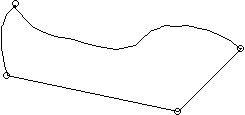
Figure 13 shows another graph with 4 vertices and 4 edges but it is not isomorphic to the graphs in Figures 9, 11, 12.
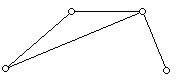
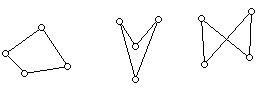
If graphs have the same structure it seems natural that their essential properties would be the same. Thus, isomorphic graphs would have the same number of vertices and edges. They would also have the same numbers occurring as the valences of the vertices of the graphs. Figure 8 has vertices of valence 2, 2, 2, 2. Figure 13 has vertices of valence 3, 2, 2, 1. Hence, the graphs in these figures are not isomorphic. Having the same valences does not, however, guarantee that there is an isomorphism between two graphs. All three of the graphs in Figure 14 look different. However, they all have valences 4, 4, 2, 2, 2, 2,
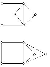
Two of the graphs in Figure 14 are isomorphic to each other but not to the third graph. Can you tell which two graphs are isomorphic? The two graphs in Figure 14 which are isomorphic as graphs have a sense in which they are not the same. Whenever, one has items which can be distinguished from each other because of additional attributes that were not previously contemplated, one has made progress.
It may be helpful to consider a situation outside of mathematics to understand the importance of words and of refining the meaning of words. One of the most important attributes of objects to people who are not color- blind is the phenomenon of color. Color is an amazingly complex subject with issues involving the physics of light, the way the eye perceives color, and linguistic issues. For example, there are languages where there are no separate words to distinguish between blue and green. Furthermore, distinctions are made between the terms color, hue, and saturation. The point is that when an author can distinguish in a novel between azure and sky blue, it enriches the experience of reading. Similarly, geometry is enriched when we are can make new distinctions between objects we think of as being familiar. For example, most of the polygons we tend to see that are drawn in the plane are convex. So making the distinction between convex polygons and non-convex polygons broadens our perspective. Now, non-convex polygons be classified according to whether they have edges that intersect themselves (at places other than vertices) or not. Figure 15 shows a convex polygon, one which is not convex and one which intersects itself, and is also not convex. All of these polygons are 4-gons.
The diagram in Figure 16 shows a geometric object that has a lot in common with a polygon but is not a polygon. Sometimes this type of geometric figure is referred to as a polygon with holes - in this example one hole. In fact, so far, a definition for what a polygon is has not been given! Based on these discussions how might you define the word polygon?

Do Now 2:
a. How would you define the concept of polygon so that all of the examples in Figure 15 but not the example in Figure 16 would be polygons?
b. Draw a variety of polygons which illustrate the ideas of being convex, non-convex, and self-intersecting.
c. Give some ideas about how to distinguish between polygons which go beyond the distinctions of being convex, non-convex, and self-intersecting.
Hint: i. What can you say about side lengths and angle lengths of polygons?
ii. What can you say about angle "types" (e.g. acute, right, obtuse) of polygons?
d. Our discussion has dealt with polygons that can be drawn in a plane. What ideas do you have about how to extend this discussion to 3-dimensional and higher dimensional spaces?
e. A common word used in connection with polygons is "regular." How would you define what it means to be a regular polygon?