Techniques for Proving Combinatorial Theorems about 3-Polytopes

Joseph Malkevitch
Department of Mathematics and Computing
York College (CUNY)
Jamaica, New York 11451

email:

malkevitch@york.cuny.edu

web page:

http://york.cuny.edu/~malk/

Convex 3-dimensional polyhedra (3-polytopes) are an important class of mathematical objects with many applications both within and outside of mathematics. Rather surprisingly, it is not necessary to be able to work with or visualize such polyhedra in 3-dimensions because from a combinatorial point of view, we can identify 3-polytopes with a special class of graphs (diagrams with dots and lines). This amazing result is due to Ernst Steinitz (1871-1928) and is often referred to as Steinitz's Theorem. However, its formulation in a way that makes it particularly useful is due to Branko Grünbaum (1929- ) and Theodore Motzkin (1908-1970).

Steintiz's Theorem (Version 1)

A graph G is 3-polytopal, that is, the vertex-edge graph of a 3-dimensional convex polyhedron if and only if G is planar and 3-connected.

Steinitz's Theorem complements the other critical tool for work with 3-polytopes, Euler's Polyhedral Formula, due to Leonhard Euler (1707-1783). This result, in its graph theory form (due to Cauchy (1789-1757)) states that for a plane connected graph V + F - E = 2 where V, F, and E denote, respectively, the number of vertices, faces, and edges of the graph. The same formula holds for the vertices, faces, and edges of a convex polyhedron.

A graph is called planar if an isomorphic copy of the graph can be drawn in the (Euclidean) plane so that the edges which join the vertices only meet (intersect) at vertices. A graph is called 3-connected if for every pair vertices u and v there are at least three paths from u to v whose only vertices (or edges) in common are u and v.

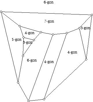
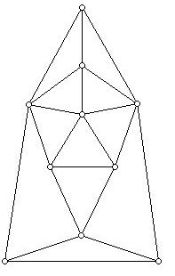
Invoking this theorem allows us to say there is a convex 3-dimensional polyhedron corresponding to Figures 1 and 2. For Figure 1 the number of sides for each face of the polyhedron is indicated for each of the faces, including the unbounded or "infinite" face, which is a 6-gon. While sometimes it may be easy to visualize a 3-dimensional polyhedron having a given plane graph, in many cases this is very difficult. Yet by Steinitz's Theorem such a polyhedron will have to exist.

Figure 2 (A plane 3-connected graph.)

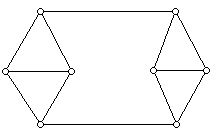
In Figure 3 we see a graph which has been drawn in the plane but is not 3-polytopal, and, thus, corresponds to no convex polyhedron because it has pairs of vertices which can only be joined by two paths. Figure 3 does, however, correspond to a non-convex 3-dimensional polyhedron.

Figure 3 (A plane graph which is not 3-polytopal.)

While Steinitz's Theorem is becoming better known, it is not as widely known that there is a "constructive" approach to Steinitz's Theorem that is often very useful. This result, rooted in Steinitz's original work, is developed in Grünbaum's book Convex Polytopes (1967).

Steinitz's Theorem (Version 2)

Every 3-polytopal graph can be obtained from the graph of the tetrahedron (K₄) by a sequence of three operations known as face splits (or dually vertex splits). Application of one of these operations begins with a planar 3-connected graph and results in a new planar 3-connected graph.

The easiest way to think about the three operations which I will call Steinitz Type I, Steinitz Type II, and Steinitz Type III, is to consider the diagrams below. In each case we start with a planar 3-connected graph and a particular face M in the graph, as shown in Figure 4, where the valences (degrees) of the vertices of face M must be three or more. Note that the edges emerging from the vertices that form M are not completely shown.

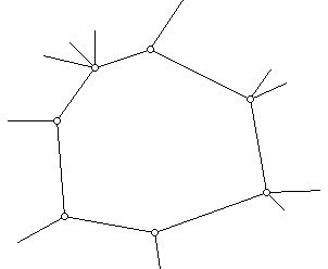
Starting with a face M such as that shown in Figure 4, we will split M into two faces but in a manner which preserves the fact that the graph obtained is still plane and 3-connected.

Figure 5 shows a Steinitz Type I operation where two existing vertices of a face (not joined by an edge, that is, not adjacent) are joined by an edge. This splits M into two faces M' and M" where the new plane 3-connected graph has one more edge and one more face and no additional vertices. Thus, Euler's Polyhedra Formula continues to hold.

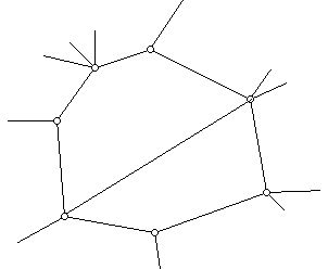
Figure 6 shows the result of a Steinitz Type II operation. Here, a new vertex is used to subdivide an existing edge of M (denoted with a "square" rather than a "circle" in Figure 6) into two edges; this new vertex is joined to an existing vertex. Again, Euler's Polyhedral Formula continues to hold and planarity and 3-connectedness are preserved. Note that the new vertex added must be 3-valent, so if this operation is done on a graph all of whose vertices have the same valence, the new graph can no longer have that property.

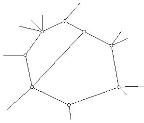
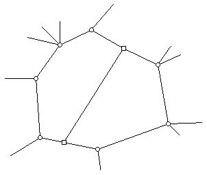
Figure 7 shows our final Steinitz operation, that of Type III. For this operation we take two edges of the face M and subdivide each of these edges using a vertex and then join these two new vertices with an edge. Both of the new vertices added are 3-valent. Thus, the only time that a Steinitz operation will preserve the fact that all the vertices of the new graph have the same valence as the vertices of the old graph is in the case of the Type III operation. The original graph is 3-valent.

The tetrahedron has 6 edges but it follows from the fact that every 3-polytope can be obtained from the tetrahedron by one of the Steinitz Operations that no 3-polytope has 7 edges.

Among the remarkable applications that Steinitz's Theorem can be put to use with are Eberhard's Theorem and Mani's Theorem.

Victor Eberhard (1861-1928) was a blind 19th century geometer who proved a kind of converse to Euler's Polyhedra Formula. Given P a 3-valent 3-polytope (or its graph G(P), then if p_i denotes number of faces of P with i sides, Euler's Polyhedral Formula states that the values p_k satisfy :

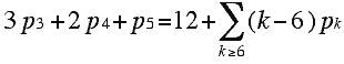
This collection of p_k will be referred to as the face vector of P. It is very easy to see there are non-negative integer values for the p_k but there is no 3-dimensional polytope Q with p_k(Q) = p_k possible.

Note that there is no restriction on the number of hexagonal faces involved because the coefficient of p₆ is zero. This means that two different polytopes can have identical face vectors except for the value of the number of hexagons in the face vector. What Eberhard showed was that if one has a collection of non-negative integers obeying the equation above, say p_k*, for k=3, 4, 5, 7, ..., n then one can choose a p₆* which is a non-negative integer and construct a 3-dimensional polytope Q* such that p_k(Q) = p_k* for k = 3, 4, 5, 6, 7, ...., n. This value for p₆* can conceivably be zero but sometimes the value must be positive.

The proof that Eberhard gave for his theorem was not rigorous by today's standards, but using Steinitz's Theorem the problem is reduced to working with planar 3-valent 3-connected graphs. One approach to using Steinitz's Theorem for a proof was given by Grünbaum, who also generalized Eberhard's Theorem to the case of 4-valent graphs and in a variety of other directions. One interesting result he shows, using Steinitz's Theorem is that if we are seeking 3-valent polytopes that have no 3-gons or 4-gons, the number of hexagons one needs to use in proving Eberhard's Theorem is never more than 8. When 3-gons and 4-gons are allowed, the number of hexagons that might be required can be shown not to be uniformly bounded.

Many of the proofs in this use the following tool in addition to Steintiz's Theorem for problems involving 3-valent graphs.

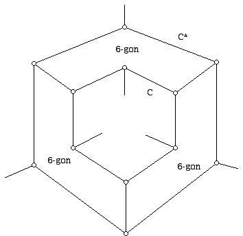
Consider the circuit C which is to be thought of as a simple closed circuit in a plane graph G. Since the graph we are thinking about is 3-valent, at each vertex as we move along C, say in the clockwise direction, there will be one other edge at each vertex other than the two in the circuit C at that vertex. In Figure 8 we have such a circuit C where the edges at the vertices we encounter alternately lie in the exterior and interior of C. If we code a vertex whose additional edge goes into the exterior of C with a 1 and a vertex whose additional edges go into the interior of C with a 0, then for the circuit C in Figure 8 we would have the cyclic code 101010. (The pattern could equally well be designated 010101.) We could write this(10)³. Surrounding the circuit C in Figure 8 is a "layer" of hexagonal faces which leads to a new circuit C*. This layer in Figure 8 consists of 3 hexagons. If we had an analogous diagram whose code was (10)^k, then we would have for this diagram a layer with k hexagons. The intriguing thing to notice is that code for C* (Figure 8) will also be (10)^k. This means that if one can find the code (10)^k in a planar 3-connected graph which is 3-valent, one can construct another planar 3-connected graph (hence, 3-polytopal!) which has the same face vector as the planar 3-connected graph one started with but which has more hexagons.

Peter Mani's Theorem deals with the relationship between the automorphism group of a plane 3-connected graph G and the symmetry of the different polyhedra that can realize this graph.

Mani's Theorem

If G is the automorphism group of the planar 3-connected graph H, there exists a 3-dimensional polyhedron P(H) which has H as its edge-vertex graph and such that the group of isometries of P(H) is isomorphic to G.

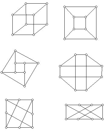
Figure 9 shows many isomorphic graphs (not all of them plane) which are isomorphic to any graph which realizes the combinatorial type of the cube (1x1x1 cube) in 3-space. All of these graphs have the same automorphism group, that is, maps of the vertex set of the graph onto itself that preserve edges. This group has order 48 (there are many groups of order 48) and is sometimes denoted O_h. What Mani's Theorem says is that there is a particular combinatorial cube which also has O_h as its isometry group. This is "our friend" the 1x1x1 cube, whose faces are all squares. If we start with a square pyramid (there are many inequivalent such polytopes) and cut of the apex (the 4-valent vertex) in different ways, we get combinatorial cubes. However, none of these polyhedra (or any other combinatorial cubes) ever have O_h as their symmetry group!

It is tempting to think that if one has a subgroup of the group O_h, the full symmetry group of the graph of the cube, for any subgroup L of this group one can also find a 3-polytope combinatorial equivalent to the cube with L as its isometry group. This is false! In fact, if one picks the rotation subgroup of O_h which is S₄ (the symmetric group on 4 letters), then there is no combinatorial cube with this as its isometry group. The same situation occurs for metrical polygons and their graphs. A square drawn in the plane has as its graph the cycle of length 4 whose symmetry group is the dihedral group with 8 elements. However, the rotation subgroup of order 4 of this dihedral group can not be realized in the plane by any metrical convex quadrilateral with exactly 4 symmetries!

Note also that different drawings of a graph (Figure 10) can have different symmetry groups as drawings in the plane.

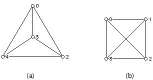
Figure 10 (a) has as a graph the group S₄ which has order 24 as its automorphism group but as a metrical drawing its symmetry group has order 6. As a metrical object Figure 10 (b) only has 8 symmetries. Note that as drawn in Figure 10 (a), we have a plane graph, while the drawing in Figure 10 (b) is not plane.

Some of the many types of combinatorial structures/concepts that be addressed using the tools above are:

a. Hamiltonian circuits

b. Hamiltonian paths

c. Pancyclicity and almost pancyclicity

d. Matchings

e. Eulerian circuits

f. Eulerian paths

and they can be looked at for special classes of graphs:

a. 3-valent

b. 4-valent

c. 5-valent

e. fullerenes

f. polyhedra with k-gons and triangles

g. polyhedra with k-gons and 4-gons

h. polyhedra with k-gons and 5-gons

and the duals of these types of objects.


References:

1. B. Grünbaum, Convex Polytopes, (2nd edition), Springer-Verlag, NY, 2003.

2. B. Grünbaum and T. Motzkin, On polyhedral graphs, Proc. Symp. Pure Math., Vol. 7 (Convexity), AMS, Providence, 1963, pp. 744-751.

3. B. Grünbaum and T. Motzkin,, The number of hexagons and the simplicity of geodesics on certain polyhedra, Can. J. Math., 15 (1963) 744-751.

4. Malkevitch, J., Polytopal Graphs. Selected Topics in Graph Theory 3, eds., L. Beineke and R. Wilson, Academic Press, NY, 1988, pp. 169-188.

5. Mani, P. Automophismen von polyedrischen Graphen, Math. Ann. 192 (1971) 279-303.

6. O. Schramm, How to cage an egg, Inventiones Mathematicae 107 (1992) 543–560,

7. E. Steinitz, Polyeder und Raumeinteilungen, Encyclopädie der mathematischen Wissenschaften, Band 3 (Geometries), 1922, pp. 1–139 .

8. E. Steinitz and H. Rademacher, Vorlesungen über die Theorie der Polyeder, Springer-Verlag, Berlin, 1934.

9. G. Ziegler, Lectures on Polytopes, Springer, NY, 1998.